Basic operations inside Jupyter

Adding a cell above the current one: ‘a’

Adding a cell below the current one: ‘b’

Delete cell entirely: ‘d,d’ (press d twice)

To execute/run a cell: Ctrl + Enter

To execute/run a cell and move to the next one: Shift + enter

Each cell has a type associated with it: “Code”, “Markdown”, “Raw”

Import libraries

import numpy as np
import matplotlib.pyplot as plt

Basic math

b = 1 + 1
print(b)

2

c = 4 * 4 # multiply
print(c)
c = 4 **2 # exponentiate
print(c)

16
16

Plotting using matplotlib package

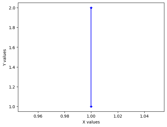
plt.plot([1,1],[1,2],'-*b') ## x array, y array and line or marker specifications
plt.xlabel('X values')
plt.ylabel('Y values')

Text(0, 0.5, 'Y values')

Numerical operation using numpy package

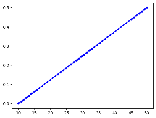
a = np.linspace(10,50,num=50) ## create a regular-spaced array from start to end and number of datapoints

b = np.linspace(0,0.5,num=50) ## create a regular-spaced array from start to stop (excluding) with step size as input

np.max(a)

50.0

np.max(b)

0.5

plt.plot(a,b,'-*b')

[<matplotlib.lines.Line2D at 0x7f405c47c700>]

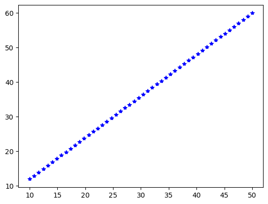
b = np.linspace(12,60,num=50)
plt.plot(a,b,'*b')

[<matplotlib.lines.Line2D at 0x7f405c3ff760>]

np.random.rand(15)

array([0.70626747, 0.79493321, 0.91271779, 0.7257214 , 0.38670769,
       0.76199924, 0.42003926, 0.26578924, 0.13720258, 0.33968749,
       0.91707911, 0.79310182, 0.1508091 , 0.98856123, 0.74599607])

np.random.randint(50,high=100,size=12)

array([65, 73, 56, 56, 64, 85, 71, 56, 53, 85, 79, 71])

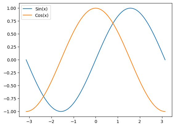
## did some plotting with sinx, cosx
x = np.linspace(-np.pi, np.pi, 100)
y = np.sin(x)
plt.plot(x, y,label='Sin(x)')
y = np.cos(x)
plt.plot(x, y, label='Cos(x)')
plt.legend()

<matplotlib.legend.Legend at 0x7f405c3c5910>

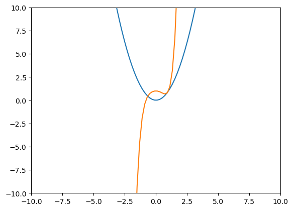
## did some plotting with polynomials
x = np.linspace(-10,10,100)
y = x ** 2
plt.plot(x, y, label ='x^2')
y = x ** 5 - x **2 + 1
plt.plot(x, y, label = 'x^5 - x^2 + 1')

## something that we did not cover in class:
plt.xlim([-10,10]) ## restricts the x-axis limit from -10 to +10
plt.ylim([-10,10]) ## restricts the y-axis limit from -10 to + 10

(-10.0, 10.0)

Installing CoolProp and calculating Enthalpy of Vaporization

install CoolProp by using:

!pip install CoolProp

or

import sys !{sys.executable} -m pip install CoolProp

from CoolProp.CoolProp import PropsSI

# enthalpy of vaporization example
H_L = PropsSI('H', 'P', 101325, 'Q', 0, 'water')
H_V = PropsSI('H', 'P', 101325, 'Q', 1, 'water')

print("the enthalpy of vaporization at P = 1 atm is:",round((H_V - H_L)/1000), 'kJ/kg')

the enthalpy of vaporization at P = 1 atm is: 2256 kJ/kg