3.4 Isobaric-Isochoric process: Nitrogen as Ideal gas

Consider \(1\:kg\) of Nitrogen stored in a piston-cylinder system sitting at atmospheric pressure and temperature (\(101\:kPa\) and \(25 ^{\circ} C\)). The system undergoes a thermodynamic cycle where its pressure is doubled through an isothermal process. Following the isothermal compression comes an isobaric expansion followed by an isochoric process to get Nitrogen to its initial state at \(101\:kPa\) and \(25 ^{\circ} C\). Assuming Nitrogen to be ideal gas, plot P-V, P-T, and T-V diagrams for this process.

Solution Approach

Let’s associate each state with a number to be able to progess in an organized way.

The initial state being (1) where

\(P_1=101\:kPa\) and \(T_1=25^{\circ} C\)

Followed by an isothermal process where the pressure is doules to reach state (2) where

\(P_2=2P_1\) and \(T_2=T_1=25^{\circ} C\)

Followed by an isobaric process to reach point (3) where

\(P_3=2P_2\)

and

\(V_3=V_1\)

because the following process from (3) back to (1) is isochoric where the volume keeps constant.

To Calculate \(V_1\) the ideal gas equation of state shall be used where

\(V=mRT/P\)

#defining variables and looking up tables
R = 0.2968 #Nitrogen gas constant in kJ/kg.K
m = 1 #mass of Nitrogen in kg
T_1 = 25 + 273.15 #temperature of Nitrogen in K
P_1 = 101 #pressure of Nitrogen in kPa

#using ideal gas law equation of state
V_1 = m * R * T_1 / P_1 #volume of Nitrogen in m3

print('The volume of Nitrogen at its initial state is:', f"{V_1:.3f}", 'm3')

The volume of Nitrogen at its initial state is: 0.876 m3

Then Nitrogen goes through an isothermal compression to double its pressure.

given mass(\(m\)), gas constant (\(R\)) and temperature (\(T\)) are constant,

\(P_2V_2=P_1V_1=mRT_1\)(or \(T_2)\)

therefore

\(V_2=P_1V_1/P_2\)

where

\(P_2=2P_1\)

therfore

\(V_2=V_1/2\)

#calculating variables at the second state
P_2 = 2 * P_1 #pressure of Nitrogen in kPa
T_2 = T_1 #temperature of Nitrogen in K
V_2 = V_1 / 2 #volume of Nitrogen in m3 at the second state
print('The volume of Nitrogen at its second state is:', f"{V_2:.3f}", 'm3')

The volume of Nitrogen at its second state is: 0.438 m3

To calculate temperature at the third state, ideal gas equation of state is to be used as

\(T_3=P_3V_3/{mR}\)

##calculating variables at the third state
P_3 = P_2 #pressure of Nitrogen in kPa
V_3 = V_1 #volume of Nitrogen in m3 at the third state

#using ideal gas law equation of state
T_3 = P_3 * V_3 / (m * R) #temperature of air in partition a in K
print('The temperature of Nitrogen at the third state is:', T_3, 'K')

The temperature of Nitrogen at the third state is: 596.3 K

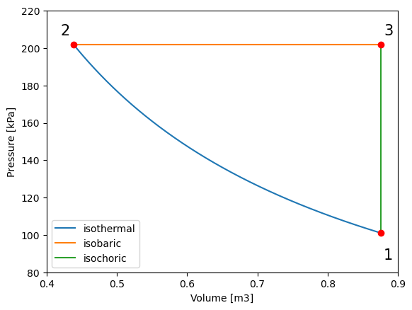
##plotting P_V
#import the libraries we'll need
import numpy as np
import matplotlib.pyplot as plt

#defining arrays of V values for 1-2
V_vals12 = np.linspace(V_1, V_2, 1000)  # define an array of values for volume (v) for the process 1 to 2
#calculating pressure (P) for the array of volume values (V_vals12)
P_vals12 = m * R * T_1 / V_vals12

#defining arrays of V values for 2-3
V_vals23 = np.linspace(V_2, V_3, 1000)  # define an array of values for volume (v) for the process 2 to 3
#associated constant pressure for the process 2-3
P_vals23 = np.linspace(P_2, P_3, 1000)

#defining arrays of P values for 3-1
P_vals31 = np.linspace(P_3, P_1, 1000)  # define an array of values for pressure (P) for the process 2 to 3
#associated constant volume for the process 3-1
V_vals31 = np.linspace(V_3, V_1, 1000)

plt.plot(V_vals12, P_vals12,label='isothermal')  # plot pressure vs. volume
plt.plot(V_vals23, P_vals23,label='isobaric')
plt.plot(V_vals31, P_vals31,label='isochoric')
plt.legend()

plt.ylabel("Pressure [kPa]")  # give y axis a label
plt.xlabel("Volume [m3]")  # give x axis a label

#add-ons to illustrate process path
plt.xlim(0.4, 0.9)
plt.ylim(80, 220)
plt.text(0.88, 87, '1', fontsize = 15)
plt.text(0.42, 207, '2', fontsize = 15)
plt.text(0.88, 207, '3', fontsize = 15)
plt.plot(V_vals12[0], P_vals12[0], 'ro')
plt.plot(V_vals23[0], P_vals23[0], 'ro')
plt.plot(V_vals31[0], P_vals31[0], 'ro')

[<matplotlib.lines.Line2D at 0x7f33cbd53af0>]

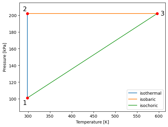
##plotting P_T
#defining arrays of T values for 1-2
T_vals12 = np.linspace(T_1, T_2, 1000)  # define an array of values for temperature (T) for the process 1 to 2

#defining arrays of T values for 2-3
T_vals23 = np.linspace(T_2, T_3, 1000)  # define an array of values for temperature (T) for the process 2 to 3

#defining arrays of T values for 3-1
T_vals31 = np.linspace(T_3, T_1, 1000)  # define an array of values for temperature (T) for the process 3 to 1

plt.plot(T_vals12, P_vals12,label='isothermal')  # plot pressure vs. volume
plt.plot(T_vals23, P_vals23,label='isobaric')
plt.plot(T_vals31, P_vals31,label='isochoric')
plt.legend()

plt.ylabel("Pressure [kPa]")  # give y axis a label
plt.xlabel("Temperature [K]")  # give x axis a label

#add-ons to illustrate process path
plt.xlim(280, 615)
plt.ylim(85, 215)
plt.text(288, 93, '1', fontsize = 15)
plt.text(288, 205, '2', fontsize = 15)
plt.text(604, 200, '3', fontsize = 15)
plt.plot(T_vals12[0], P_vals12[0], 'ro')
plt.plot(T_vals23[0], P_vals23[0], 'ro')
plt.plot(T_vals31[0], P_vals31[0], 'ro')

[<matplotlib.lines.Line2D at 0x7f33cb4bf7f0>]

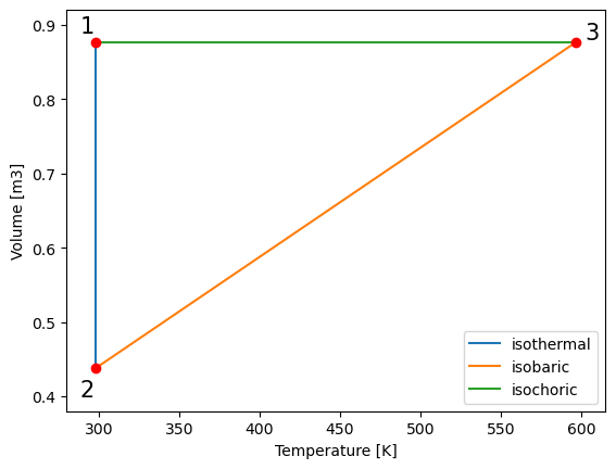
##plotting T_V

plt.plot(T_vals12, V_vals12,label='isothermal')  # plot pressure vs. volume
plt.plot(T_vals23, V_vals23,label='isobaric')
plt.plot(T_vals31, V_vals31,label='isochoric')
plt.legend()

plt.ylabel("Volume [m3]")  # give y axis a label
plt.xlabel("Temperature [K]")  # give x axis a label

#add-ons to illustrate process path
plt.xlim(280, 615)
plt.ylim(0.38, 0.92)
plt.text(288, 0.89, '1', fontsize = 15)
plt.text(288, 0.40, '2', fontsize = 15)
plt.text(602, 0.88, '3', fontsize = 15)
plt.plot(T_vals12[0], V_vals12[0], 'ro')
plt.plot(T_vals23[0], V_vals23[0], 'ro')
plt.plot(T_vals31[0], V_vals31[0], 'ro')

[<matplotlib.lines.Line2D at 0x7f33cb45e580>]