3.3 Piston-cylinder system for Air

Problem Statement

Consider \(2\:kg\) air at \(200\:kPa\) and \(25 ^{\circ} C\) stored in a cylinder-piston system which is in thermal equilibrium with its surrounding. Assuming air at this state as ideal gas,

a) calculate how much space does air occupy in this state.

b) if the piston is moved to compress air to half its initial volume at constant temperature, calculate the final air pressure.

c) plot the process on P-V, P-T and T-V diagrams.

Solution Approach for a)

Ideal gas equation can be used as EOS since the assumption is valid as per the statement, so

\(PV=mRT\)
\(V=mRT/P\)

#defining variables and looking up tables
R = 0.287 #air gas constant in kJ/kg.K
m = 2 #mass of air in kg
T = 25 + 273.15 #temperature of air in K
P = 200 #pressure of airc in kPa

#using ideal gas law equation of state
V_1 = m * R * T / P #volume of air in m3

print('The air volume is:', round(V_1,3), 'm3')

The air volume is: 0.856 m3

Solution Approach for b)

The box is compressed to half its initial volume therefore \(V_2=V_1/2\) and temperature remains constant as per the question’s statement.

Ideal gas equation solved for pressure (P) is to be used to calculate pressure.

\(P=mRT/V\)

V_2 = V_1 / 2 #volume of air after compression

#using ideal gas law equation of state
P_2 = m * R * T / V_2 #final pressure of the mixture in kPa
print('Secondary air pressure is:', P_2, 'kPa')

Secondary air pressure is: 400.0 kPa

Solution Approach for c)

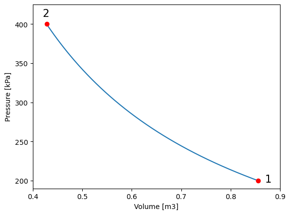
for a P-v diagram, the ideal gas equation is to be used in a form in which pressure(\(P\)) and volume(\(v\)) are the variables calculated one based on the other one.

\(P=mRT(1/V)\)

where mRT would be a constant value

#import the libraries we'll need
import numpy as np
import matplotlib.pyplot as plt

#building a range for volume (v) so that pressure (P) is calculated based upon 
V_max = V_1 #maximum amount for volume in the process
V_min = V_2 #minimum amount for volume in the process
V_vals = np.linspace(V_min, V_max, 1000)  # define an array of values for volume (v)

#calculating pressure (P) for the array of volume values (V_vals)
P_vals = m * R * T / V_vals

plt.plot(V_vals, P_vals)  # plot pressure vs. volume
plt.ylabel("Pressure [kPa]")  # give y axis a label
plt.xlabel("Volume [m3]")  # give x axis a label


#add-ons to illustrate process path
plt.xlim(0.4, 0.9)
plt.ylim(190, 425)
plt.text(0.87, 198, '1', fontsize = 15)
plt.text(0.42, 410, '2', fontsize = 15)
plt.plot(V_vals[0], P_vals[0], 'ro')
plt.plot(V_vals[-1], P_vals[-1], 'ro')

[<matplotlib.lines.Line2D at 0x7fe5ed496d00>]

#building temperature range to plot P-T and V_T diagrams
T_C = T - 273.15 #process temperature in Celsius
T_vals = np.linspace(T_C, T_C, 1000)  # define an array of values for temperature (T)
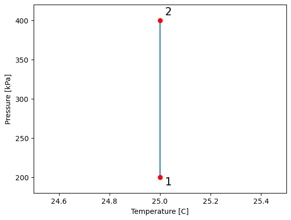
plt.plot(T_vals, P_vals)  # plot pressure vs. temperature
plt.ylabel("Pressure [kPa]")  # give y axis a label
plt.xlabel("Temperature [C]")  # give x axis a label

#add-ons to illustrate process path
plt.xlim(24.5, 25.5)
plt.ylim(180, 420)
plt.text(25.02, 190, '1', fontsize = 15)
plt.text(25.02, 407, '2', fontsize = 15)
plt.plot(T_vals[0], P_vals[0], 'ro')
plt.plot(T_vals[-1], P_vals[-1], 'ro')

[<matplotlib.lines.Line2D at 0x7fe5ecbe8d60>]

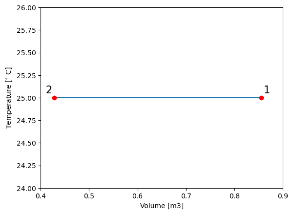
plt.plot(V_vals,T_vals)  # plot volume vs. temperature
plt.ylabel("Temperature [$^{\circ}$ C]")  # give y axis a label
plt.xlabel("Volume [m3]")  # give x axis a label

#add-ons to illustrate process path
plt.xlim(0.4, 0.9)
plt.ylim(24, 26)
plt.text(0.86, 25.05, '1', fontsize = 15)
plt.text(0.41, 25.05, '2', fontsize = 15)
plt.plot(V_vals[0], T_vals[0], 'ro')
plt.plot(V_vals[-1], T_vals[-1], 'ro')

[<matplotlib.lines.Line2D at 0x7fe5ecbe2b50>]