6.11 Second Law for an Open Turbine#
Problem Statement:#
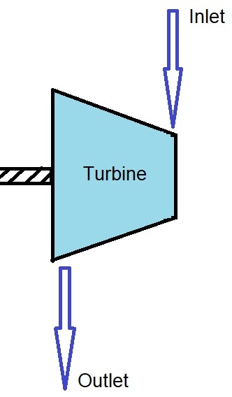
\(1\:kg/s\) of steam enters a turbine at a pressure \(P=5\:MPa\) and temperature \(T=600\:^{\circ}C\) and leaves the turbine at a pressure \(P=1\:MPa\) and temperature \(T=500\:^{\circ}C\).
assuming an insulated turbine calculate:
a) work output
b) entropy generation
assuming the outlet temperature to change to \(T=300\:^{\circ}C\) at the same pressure, calculate:
c) work output
d) entropy generation (is this feasible?)
assuming a less ideal turbine losing \(\dot Q=250\:kW\) of heat at an interface temperature of \(T_{surr}=100^{\circ}C\) to the environemnt while the outlet temperature assumption \(T=300\:^{\circ}C\) persists, calculate:
e) work output
f) entropy generation (is this feasible?)
Solution Approach for a)#
from the firt law
\(\dot Q+\dot m_ih_i=\dot W+\dot m_eh_e\)
since the turbine is insulated
\(\dot Q=0\)
and
\(\dot W=\dot m_ih_i-\dot m_eh_e\)
# import the libraries we'll need
import CoolProp.CoolProp as CP

#define variables
fluid = "water"  # define the fluid or material of interest

m_i = 1   #inlet mass flow-rate in kg/s
m_e = 1   #outlet mass flow-rate in kg/s

p_i = 5e+6   #inlet pressure in Pa
p_e = 2e+6   #outlet pressure in Pa
T_i = 600 + 273.15   #inlet temperature in K
T_e = 500 + 273.15   #outlet temperature in K

h_i = CP.PropsSI("H", "T", T_i, "P", p_i , fluid)   #inlet enthalpy in J/kg
h_e = CP.PropsSI("H", "T", T_e, "P", p_e , fluid)   #inlet enthalpy in J/kg

w = m_i * h_i - m_e * h_e   #specific work in W

print('The amount of work output is:', f"{w/1000:.1f}", 'kW')
The amount of work output is: 198.6 kW
Solution Approach for b)#
for an open system
\(\dot m_es_e-\dot m_is_i=\dot Q/T_{surr}+\dot S_{gen}\)
and since the turbine is insulated
\(\dot S_{gen}=\dot m_es_e-\dot m_is_i\)
s_i = CP.PropsSI("S", "T", T_i, "P", p_i , fluid)   #inlet entropy in J/kgK
s_e = CP.PropsSI("S", "T", T_e, "P", p_e , fluid)   #inlet entropy in J/kgK

s_gen = m_e * s_e - m_i * s_i   #entropy generation in W/K

print('The amount of entropy generation is:', f"{s_gen/1000:.3f}", 'KW/K')
The amount of entropy generation is: 0.173 KW/K
Solution Approach for c)#
T_e = 300 + 273.15   #outlet temperature in K

h_e = CP.PropsSI("H", "T", T_e, "P", p_e , fluid)   #inlet enthalpy in J/kg

w = m_i * h_i - m_e * h_e   #specific work in W

print('The amount of work output for 300C outlet temperature is:', f"{w/1000:.1f}", 'kW')
The amount of work output for 300C outlet temperature is: 642.7 kW
Solution Approach for d)#
s_e = CP.PropsSI("S", "T", T_e, "P", p_e , fluid)   #inlet entropy in J/kgK

s_gen = m_e * s_e - m_i * s_i   #entropy generation in W/K

print('The amount of entropy generation for 300C outlet temperature is:', f"{s_gen/1000:.3f}", 'KW/K')
The amount of entropy generation for 300C outlet temperature is: -0.492 KW/K
Solution Approach for e)#
from the firt law
\(\dot Q+\dot m_ih_i=\dot W+\dot m_eh_e\)
therefore
\(\dot W=\dot m_ih_i-\dot m_eh_e+\dot Q\)
q = -250e+3   #heat loss in W
w = m_i * h_i - m_e * h_e + q   #specific work in W

print('The amount of work output for 300C outlet temperature and 250kW heat loss is:', f"{w/1000:.1f}", 'kW')
The amount of work output for 300C outlet temperature and 250kW heat loss is: 392.7 kW
Solution Approach for f)#
for an open system
\(\dot m_es_e-\dot m_is_i=\dot Q/T_{surr}+\dot S_{gen}\)
so
\(\dot S_{gen}=\dot m_es_e-\dot m_is_i-\dot Q/T_{surr}\)
T_s = 100 + 273.15   #surrounding temperature in K

s_gen = m_e * s_e - m_i * s_i - q/T_s   #entropy generation in W/K

print('The amount of entropy generation for 300C outlet temperature and 250kW heat loss is:', f"{s_gen/1000:.3f}", 'KW/K')
The amount of entropy generation for 300C outlet temperature and 250kW heat loss is: 0.178 KW/K